This vignette will guide you to the different imputation methods HDAnalyzeR offers. First of all, we will load the package, as well as dplyr, ggplot2 and patchwork for data manipulation and visualization.
Loading the Data
Let’s start with loading the example data and metadata that come with the package and initialize the HDAnalyzeR object.
hd_obj <- hd_initialize(dat = example_data,
                        metadata = example_metadata,
                        is_wide = FALSE,
                        sample_id = "DAid",
                        var_name = "Assay",
                        value_name = "NPX")
Explore Missing Values
We can simply check our data for NA values by using the
hd_qc_summary() as we did in previous vignettes. This time
we will use something specific to NA values, the
hd_na_search() function. This function will return a
summary heatmap showing the distribution of NA values across the data
and metadata variables. This function is ideal to dive into the missing
values and understand if there are any patterns in the missing data.
This is important in order to decide how to handle them (e.g., impute or
remove).
na_res <- hd_na_search(hd_obj,
                       annotation_vars = c("Sex", "Age", "Disease"),
                       palette = list(Disease = "cancers12",
                                      Sex = "sex"),
                       x_labels = FALSE,
                       y_labels = FALSE)

na_res$na_heatmap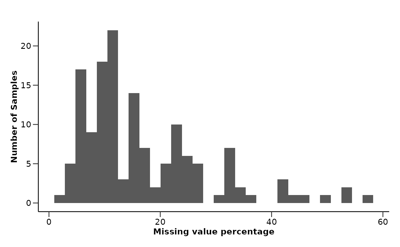
In this case, we can see that the NA values are generally spread across the different Assays, samples and metadata variables. There is a higher concentration of missing values in Myeloma that may require further investigation. In our case, we will try impute them!
Imputation Methods
Median Imputation
We will start the imputation with the simplest and fastest method,
which is the median imputation by using the
hd_impute_median(). After the imputation, we will check the
sample distribution of a random Assay that contains missing values to
see if these values are imputed logically. In a real case, this check
should be done to more than just one assay.
imputed_hd_obj <- hd_impute_median(hd_obj, verbose = FALSE)

plot_before <- hd_obj$data |>
  ggplot(aes(x = ACTA2)) +
  geom_histogram(fill = "lightblue", color = "black", alpha = 0.5, bins = 30) +
  labs(title = "Before imputation",
       x = "ACTA2", y = "Count") +
  ylim(0, 90) +
  theme_minimal()

plot_after <- imputed_hd_obj$data |>
  ggplot(aes(x = ACTA2)) +
  geom_histogram(fill = "lightpink", color = "black", alpha = 0.5, bins = 30) +
  labs(title = "After median imputation",
       x = "ACTA2", y = "Count") +
  ylim(0, 90) +
  theme_minimal()

plot_before + plot_after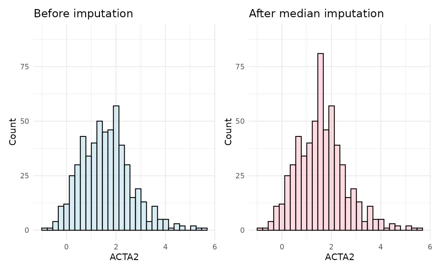
As observed in the plots, the distribution of the ACTA2 assay shifts after imputation, with an exaggerated median value in the imputed data. This highlights a key drawback of median imputation: the more missing values there are, the greater the potential bias.
KNN Imputation
A better approach is to use the hd_impute_knn() with 5
neighbors, which imputes missing values based on the 5-nearest
neighbors. We will use the same assay to compare the imputed data with
the original data.
imputed_hd_obj <- hd_impute_knn(hd_obj, k = 5, verbose = FALSE)

plot_before <- hd_obj$data |>
  ggplot(aes(x = ACTA2)) +
  geom_histogram(fill = "lightblue", color = "black", alpha = 0.5, bins = 30) +
  labs(title = "Before imputation",
       x = "ACTA2", y = "Count") +
  ylim(0, 90) +
  theme_minimal()

plot_after <- imputed_hd_obj$data |>
  ggplot(aes(x = ACTA2)) +
  geom_histogram(fill = "lightpink", color = "black", alpha = 0.5, bins = 30) +
  labs(title = "After KNN imputation",
       x = "ACTA2", y = "Count") +
  ylim(0, 90) +
  theme_minimal()

plot_before + plot_after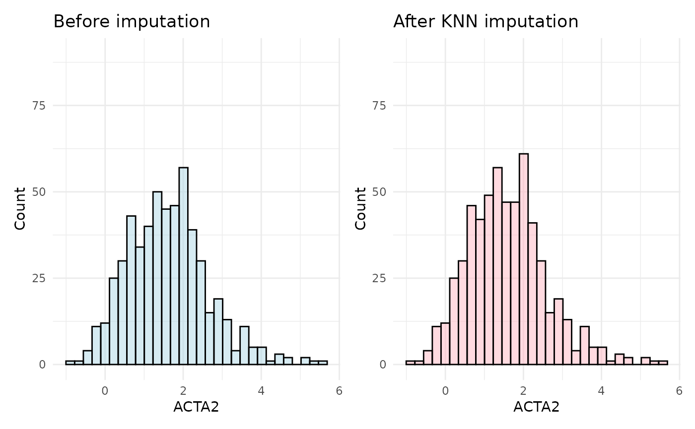
In this case, the distribution of the ACTA2 assay after imputation is more similar to the original distribution. This is because the KNN imputation method uses the nearest neighbors to impute missing values, which is more accurate and representative than median imputation.
MissForest Imputation
Finally, we will use the hd_impute_missForest() method,
which uses the random forest algorithm to impute missing values. We will
use the default values for the number of trees and the number of
iterations.
imputed_hd_obj <- hd_impute_missForest(hd_obj, verbose = FALSE)

plot_before <- hd_obj$data |>
  ggplot(aes(x = ACTA2)) +
  geom_histogram(fill = "lightblue", color = "black", alpha = 0.5, bins = 30) +
  labs(title = "Before imputation",
       x = "ACTA2", y = "Count") +
  ylim(0, 90) +
  theme_minimal()

plot_after <- imputed_hd_obj$data |>
  ggplot(aes(x = ACTA2)) +
  geom_histogram(fill = "lightpink", color = "black", alpha = 0.5, bins = 30) +
  labs(title = "After MissForest imputation",
       x = "ACTA2", y = "Count") +
  ylim(0, 90) +
  theme_minimal()

plot_before + plot_after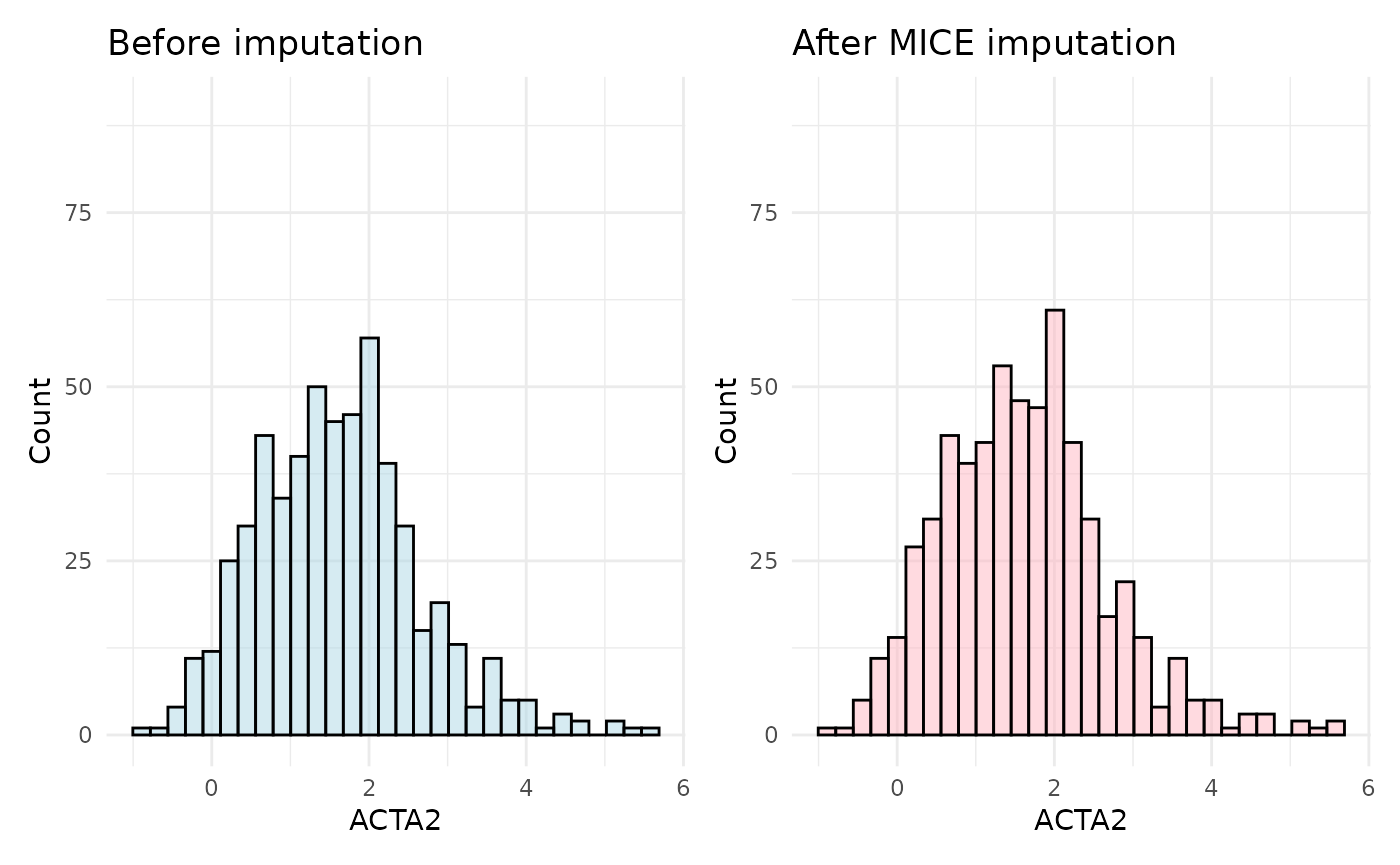
The MissForest imputation method is usually the most accurate and
also very robust, as it uses the complex random forest algorithm to
impute missing values. This method is particularly useful for large
datasets with complex relationships between variables. On the other
hand, it is by far the most computationally expensive and it would help
parallelize it. You can do that by creating and registering a cluster
with a package like doParallel and then setting the
parallelize argument to “forests” or “variables”.
📓 All methods assume that the data is missing at random, which is a common assumption in imputation methods. If the data are missing in a biased way (either technical or biological), the imputation methods may introduce bias into the data. In such cases, it is important to carefully consider the way the data were collected and what they represent.
Removing Missing Values instead of Imputing
If for any reason you do not want to impute the data, you can use the
hd_omit_na() function to easily remove the rows with
missing values in specific variables. In this example, we will remove
all rows with missing values in any of the assays.
imputed_hd_obj <- hd_omit_na(hd_obj)

plot_before <- hd_obj$data |>
  ggplot(aes(x = ACTA2)) +
  geom_histogram(fill = "lightblue", color = "black", alpha = 0.5, bins = 30) +
  labs(title = "Before imputation",
       x = "ACTA2", y = "Count") +
  ylim(0, 90) +
  theme_minimal()

plot_after <- imputed_hd_obj$data |>
  ggplot(aes(x = ACTA2)) +
  geom_histogram(fill = "lightpink", color = "black", alpha = 0.5, bins = 30) +
  labs(title = "After removing missing values",
       x = "ACTA2", y = "Count") +
  ylim(0, 90) +
  theme_minimal()

plot_before + plot_after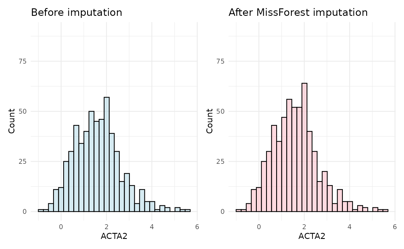
# Data after removing missing values only in specific columns
res <- hd_omit_na(hd_obj, columns = "AARSD1")
res$data
#> # A tibble: 552 × 101
#>    DAid    AARSD1  ABL1  ACAA1    ACAN    ACE2  ACOX1    ACP5    ACP6 ACTA2
#>    <chr>    <dbl> <dbl>  <dbl>   <dbl>   <dbl>  <dbl>   <dbl>   <dbl> <dbl>
#>  1 DA00001   3.39 2.76   1.71   0.0333  1.76   -0.919  1.54    2.15   2.81
#>  2 DA00002   1.42 1.25  -0.816 -0.459   0.826  -0.902  0.647   1.30   0.798
#>  3 DA00004   3.41 3.38   1.69  NA       1.52   NA      0.841   0.582  1.70
#>  4 DA00005   5.01 5.05   0.128  0.401  -0.933  -0.584  0.0265  1.16   2.73
#>  5 DA00006   6.83 1.18  -1.74  -0.156   1.53   -0.721  0.620   0.527  0.772
#>  6 DA00008   2.78 0.812 -0.552  0.982  -0.101  -0.304  0.376  -0.826  1.52
#>  7 DA00009   4.39 3.34  -0.452 -0.868   0.395   1.71   1.49   -0.0285 0.200
#>  8 DA00010   1.83 1.21  -0.912 -1.04   -0.0918 -0.304  1.69    0.0920 2.04
#>  9 DA00011   3.48 4.96   3.50  -0.338   4.48    1.26   2.18    1.62   1.79
#> 10 DA00012   4.31 0.710 -1.44  -0.218  -0.469  -0.361 -0.0714 -1.30   2.86
#> # ℹ 542 more rows
#> # ℹ 91 more variables: ACTN4 <dbl>, ACY1 <dbl>, ADA <dbl>, ADA2 <dbl>,
#> #   ADAM15 <dbl>, ADAM23 <dbl>, ADAM8 <dbl>, ADAMTS13 <dbl>, ADAMTS15 <dbl>,
#> #   ADAMTS16 <dbl>, ADAMTS8 <dbl>, ADCYAP1R1 <dbl>, ADGRE2 <dbl>, ADGRE5 <dbl>,
#> #   ADGRG1 <dbl>, ADGRG2 <dbl>, ADH4 <dbl>, ADM <dbl>, AGER <dbl>, AGR2 <dbl>,
#> #   AGR3 <dbl>, AGRN <dbl>, AGRP <dbl>, AGXT <dbl>, AHCY <dbl>, AHSP <dbl>,
#> #   AIF1 <dbl>, AIFM1 <dbl>, AK1 <dbl>, AKR1B1 <dbl>, AKR1C4 <dbl>, …
In this vignette we showed that via HDAnalyzeR you can impute your data with different methods, each of them with its own advantages and drawbacks. You can choose the method that best fits your data and your analysis needs. When using KNN or MissForest imputation methods, you should experiment with the parameters and look at the distributions of assays before and after to pick the most suitable.
📓 Remember that these data are a dummy-dataset with artificial data and the results in this guide should not be interpreted as real results. The purpose of this vignette is to show you how to use the package and its functions.