Post Analysis: Pathway Enrichment & Automated Literature Search
Source:vignettes/post_analysis.Rmd
post_analysis.RmdThis vignette will guide you through the post analysis of the results
obtained from the HDAnalyzeR pipeline. The post analysis consists of two
possible steps: pathway enrichment analysis and automated literature
search. The pathway enrichment analysis is performed using the Gene
Ontology, KEGG and Reactome databases from clusterProfiler
and ReactomePA packages respectively. The automated
literature search is performed using the the PubMed database.
If you want to learn more about ORA and GSEA, please refer to the following publications:
- Chicco D, Agapito G. Nine quick tips for pathway enrichment analysis. PLoS Comput Biol. 2022 Aug 11;18(8):e1010348. doi: 10.1371/journal.pcbi.1010348. PMID: 35951505; PMCID: PMC9371296. https://pmc.ncbi.nlm.nih.gov/articles/PMC9371296/
- https://yulab-smu.top/biomedical-knowledge-mining-book/enrichment-overview.html#gsea-algorithm
📓 Remember that these data are a dummy-dataset with artificial data and the results in this guide should not be interpreted as real results. This is why we are using extremely large p-value cutoffs in this case that should not be used in real data.
Loading the Data
We will load HDAnalyzeR and dplyr, load the example data and metadata that come with the package and initialize the HDAnalyzeR object.
library(HDAnalyzeR)
library(dplyr)

hd_obj <- hd_initialize(dat = example_data,
                        metadata = example_metadata,
                        is_wide = FALSE,
                        sample_id = "DAid",
                        var_name = "Assay",
                        value_name = "NPX")
For the Over Representation Analysis we are going to use a list of differentially expressed proteins. In this example we are going to use the up-regulated proteins. We could also use the features list from the classification models or even run both and get the intersect as it is done in the Get Started guide.
de_res <- hd_de_limma(hd_obj, case = "AML")Over Representation Analysis
First, we will perform an Over Representation Analysis (ORA) using
the Gene Ontology database and the BP ontology. We will use the
hd_ora() and hd_plot_ora() functions to run
the analysis and plot the results respectively.
proteins <- de_res$de_res |>
  filter(logFC > 0 & adj.P.Val < 0.05) |>
  pull(Feature)

enrichment <- hd_ora(proteins, database = "GO", ontology = "BP")

enrichment_plots <- hd_plot_ora(enrichment)

enrichment_plots$dotplot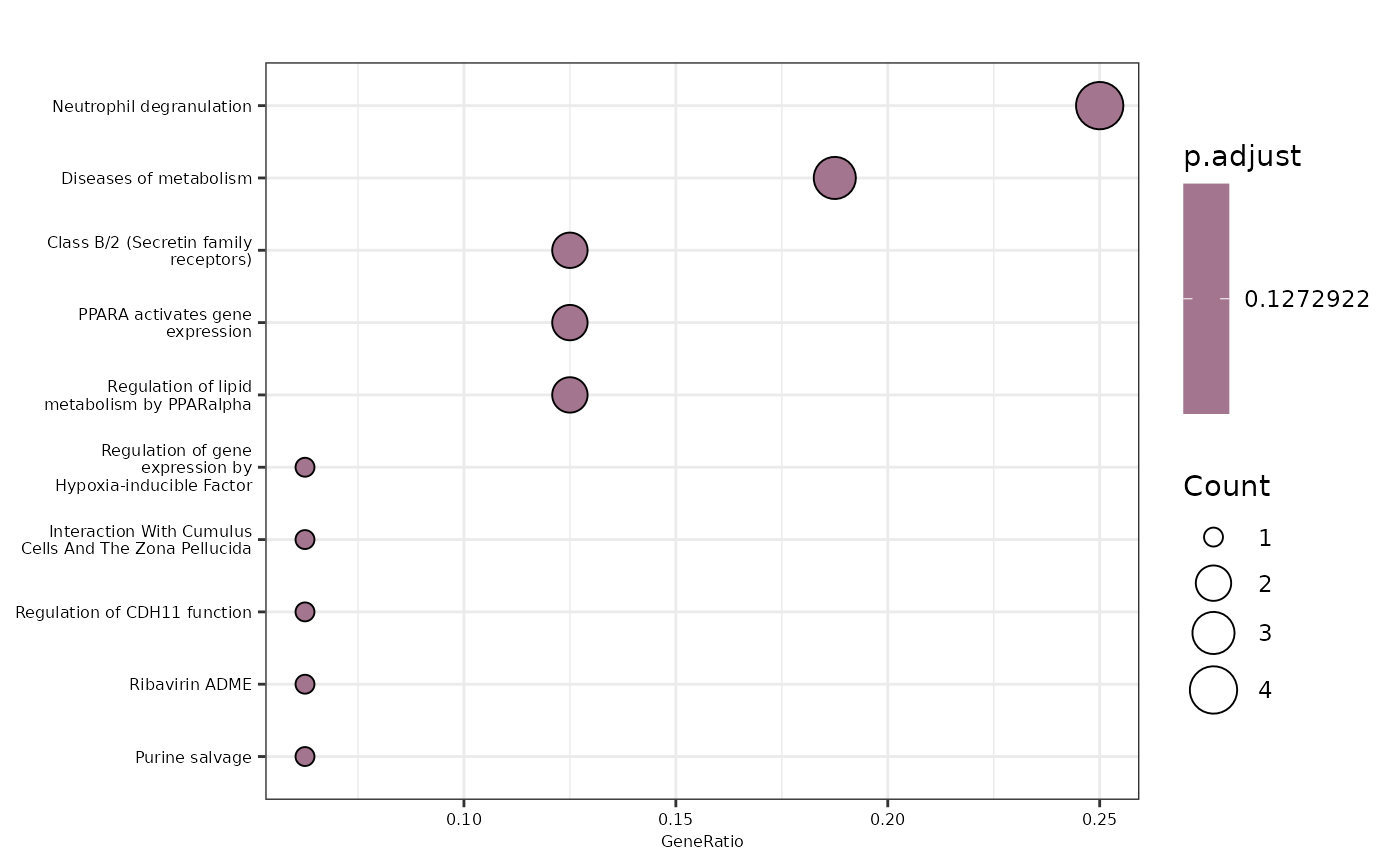
enrichment_plots$treeplot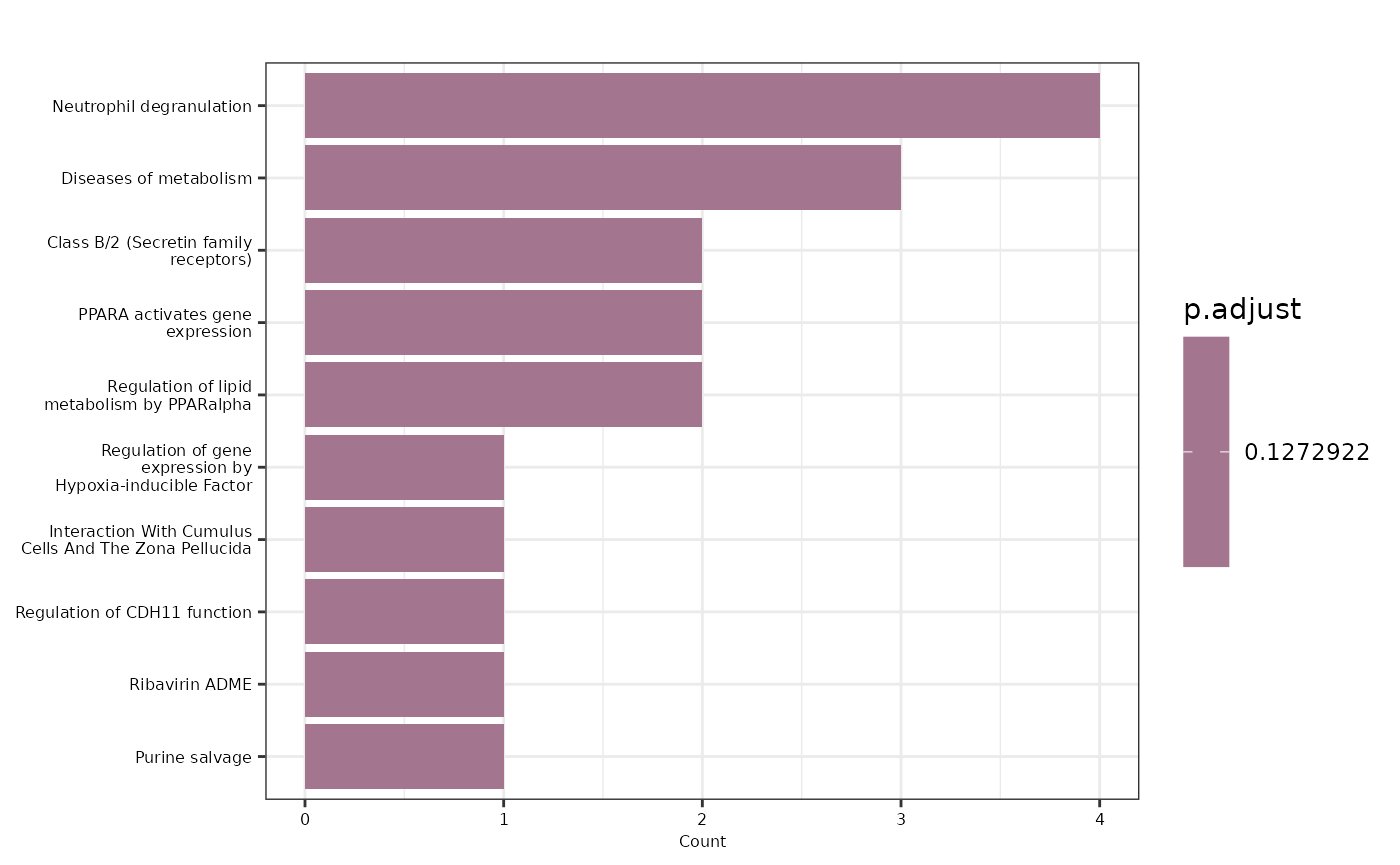
enrichment_plots$cnetplot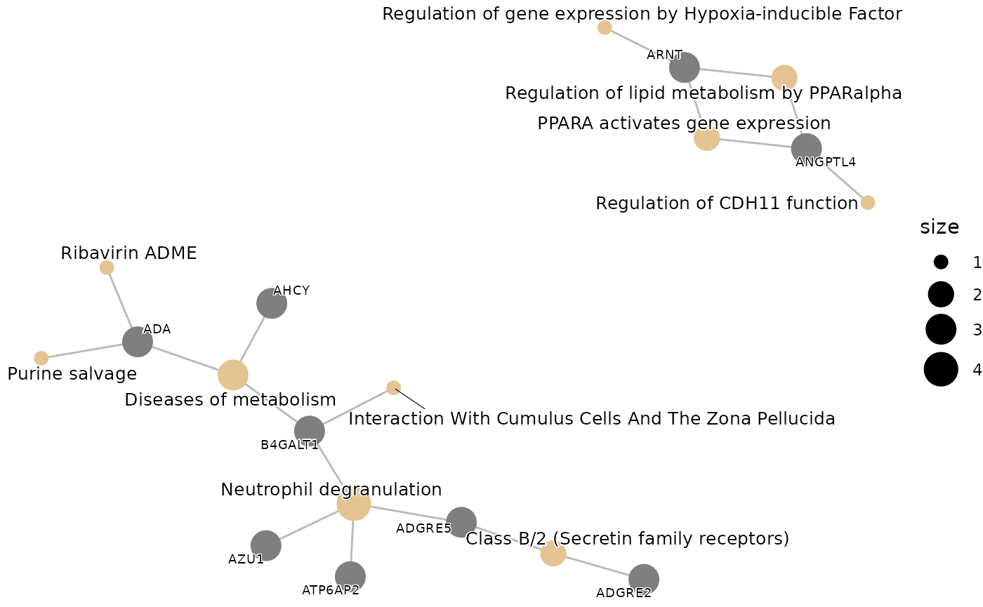
Let’s change the database and the p-value threshold.
enrichment  <- hd_ora(proteins, database = "Reactome", pval_lim = 0.2)

enrichment_plots <- hd_plot_ora(enrichment)

enrichment_plots$dotplot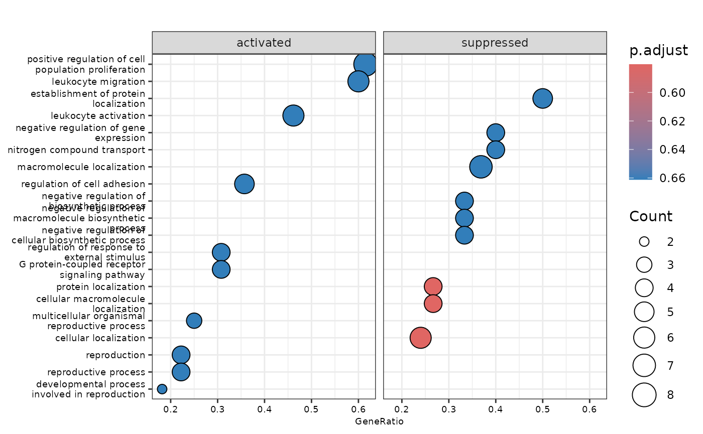
enrichment_plots$treeplot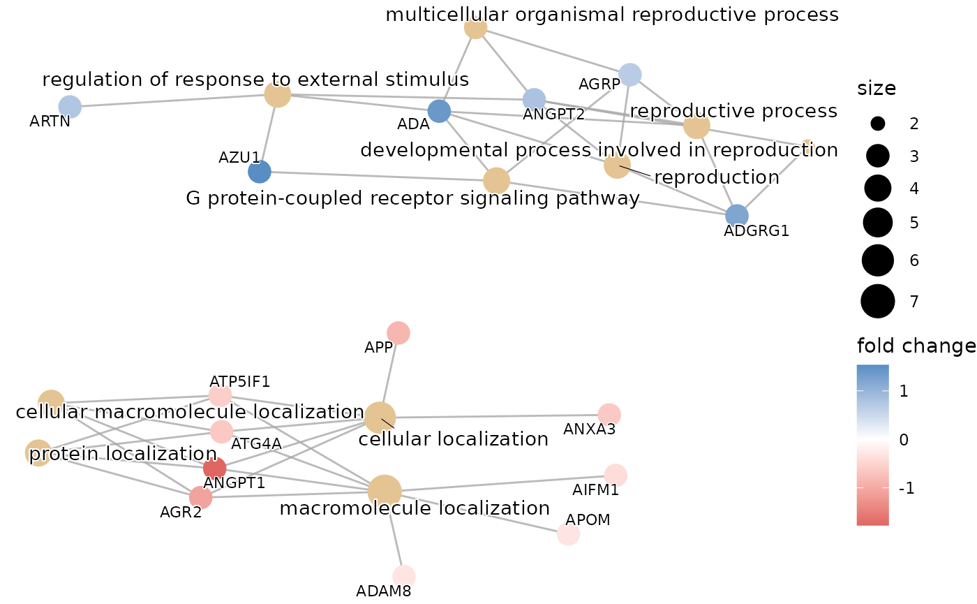
enrichment_plots$cnetplot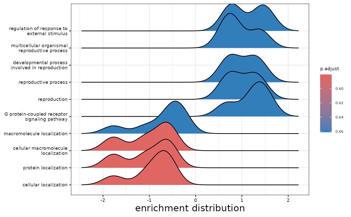
Gene Set Enrichment Analysis
We can also run a Gene Set Enrichment Analysis (GSEA) using the
hd_gsea() and hd_plot_gsea functions. The
hd_plot_gsea() function will plot the results.
⚠️ In this case, the function requires strictly differential expression results, so a ranked list of proteins is derived based on the
ranked_byargument.
enrichment <- hd_gsea(de_res, database = "GO", ontology = "BP", pval_lim = 0.55)

enrichment_plots <- hd_plot_gsea(enrichment)

enrichment_plots$dotplot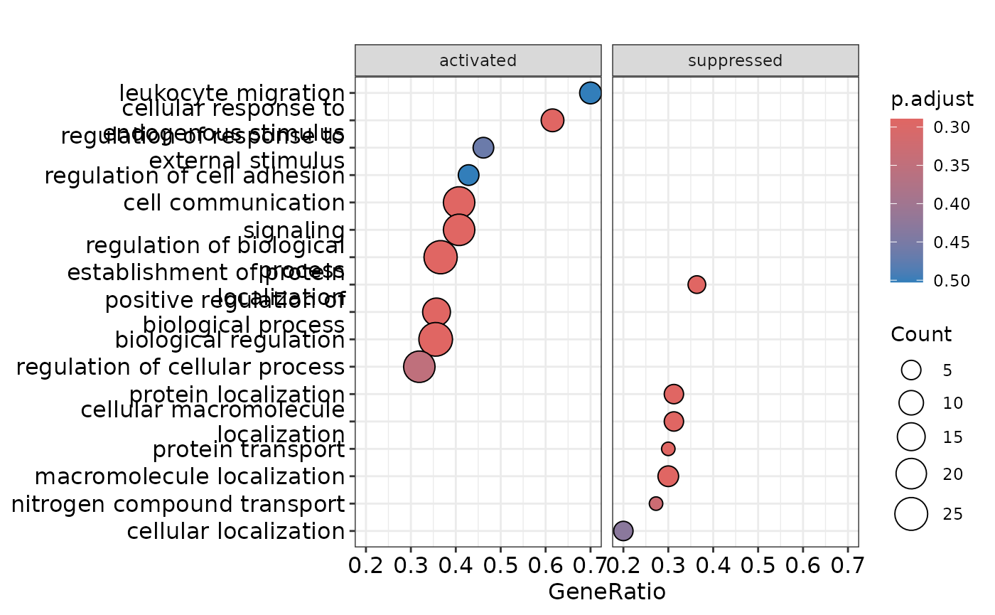
enrichment_plots$gseaplot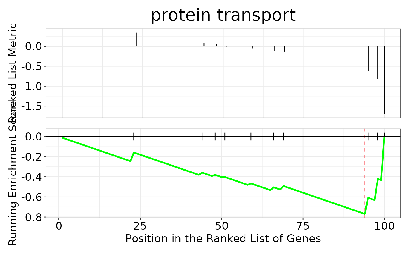
enrichment_plots$cnetplot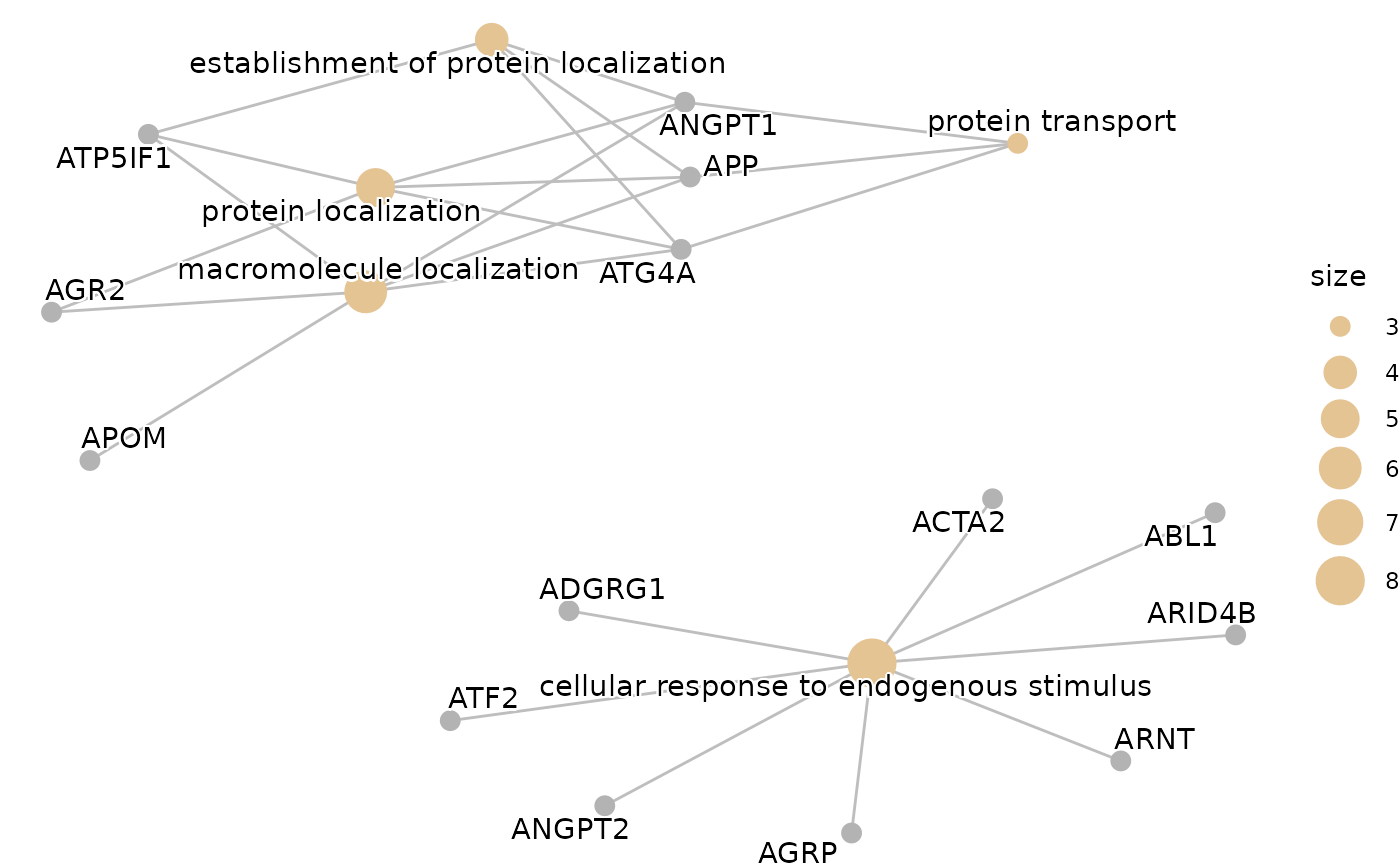
enrichment_plots$ridgeplot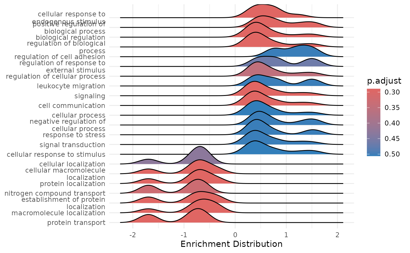
We can also change the ranking variable to the product of logFC and
-log(adjusted p value) instead of the default logFC by changing the
ranked_by argument to “both”. We could also use other
variables such as p-value or any other variable in the DE results.
However, you should use as ranking a variable that has some form of
biological relevance of the variable.
enrichment <- hd_gsea(de_res,
                      database = "GO",
                      ontology = "BP",
                      pval_lim = 0.9,
                      ranked_by = "both")

enrichment_plots <- hd_plot_gsea(enrichment)
enrichment_plots$cnetplot
Searching PubMed for our Biomarkers
Finally, let’s perform an automated literature search using the
hd_literature_search(). The function requires a list with
disease names as names and genes/proteins as values. We will create the
list, run the search and preview the results.
biomarkers <- list("acute myeloid leukemia" = c("FLT3", "EPO"),
                   "chronic lymphocytic leukemia" = c("PARP1", "FCER2"))

lit_res <- hd_literature_search(biomarkers, max_articles = 5)
#> Searching for articles on FLT3 and acute myeloid leukemia
#> Searching for articles on EPO and acute myeloid leukemia
#> Searching for articles on PARP1 and chronic lymphocytic leukemia
#> Searching for articles on FCER2 and chronic lymphocytic leukemia

lit_res$`acute myeloid leukemia`$FLT3$title
#> [1] "Supportive effect of corticosteroid on bone marrow recovery in FLT3/ITD positive acute myeloid leukemia with trisomy 13."
#> [2] "Identification of HOXA9 methylation as an epigenetic biomarker predicting prognosis and guiding treatment choice in acute myeloid leukemia."
#> [3] "Expression and clinical significance of histamine receptors in pediatric AML."
#> [4] "The improved prognosis of <i>FLT3</i>-internal tandem duplication but not tyrosine kinase domain mutations in acute myeloid leukemia in the era of targeted therapy: a real-world study using large-scale electronic health record data."
#> [5] "Oncogenic FLT3 internal tandem duplications (ITD) and CD45/PTPRC control osteoclast functions and bone microarchitecture."
📓 Remember once again that these data are a dummy-dataset with artificial data and the results in this guide should not be interpreted as real results. The purpose of this vignette is to show you how to use the package and its functions.