Run PCA analysis — do_pca • HDAnalyzeR

do_pca() runs a PCA analysis on the provided data. The function can visualize the sample points on the first and second PC plane as well as the PCA loadings and the explained variance. It can also save the plots in the results directory.

Usage

do_pca(
  olink_data,
  metadata = NULL,
  pcs = 5,
  color = "Disease",
  palette = NULL,
  wide = TRUE,
  assay = FALSE,
  impute = TRUE,
  plots = TRUE,
  x = "PC1",
  y = "PC2",
  npcs = 4,
  nproteins = 8,
  loadings = FALSE,
  save = FALSE
)

Arguments

olink_data: A tibble with the data to be used in the PCA analysis.
metadata: A tibble with metadata information to be used in the PCA plots. Default is NULL.
pcs: The number of PCs to be calculated. Default is 5.
color: The name of the column in metadata that contains the variable. to be used to plot the points color. Default is "Disease".
palette: The color palette for the plot. If it is a character, it should be one of the palettes from get_hpa_palettes().
wide: If TRUE, the data is assumed to be in wide format. Default is TRUE.
assay: If TRUE, each point is an assay and not a sample. Default is FALSE.
impute: If TRUE, the data is imputed before the PCA analysis. Default is TRUE.
plots: If TRUE, the function creates plots of the PCA results. Default is TRUE.
x: The component to be plotted on the x-axis. Default is "PC1".
y: The component to be plotted on the y-axis. Default is "PC2".
npcs: The number of PCs to be plotted. Default is 4.
nproteins: The number of proteins to be plotted. Default is 8.
loadings: If TRUE, the PCA loadings are plotted on the 2 dimensional plot. Default is FALSE.
save: If TRUE, the plots are saved in the results directory. Default is FALSE.

Value

A list with the PCA results and, if requested, the PCA plots.

pca_res: A tibble with the PCA results.
loadings: A tibble with the PCA loadings.
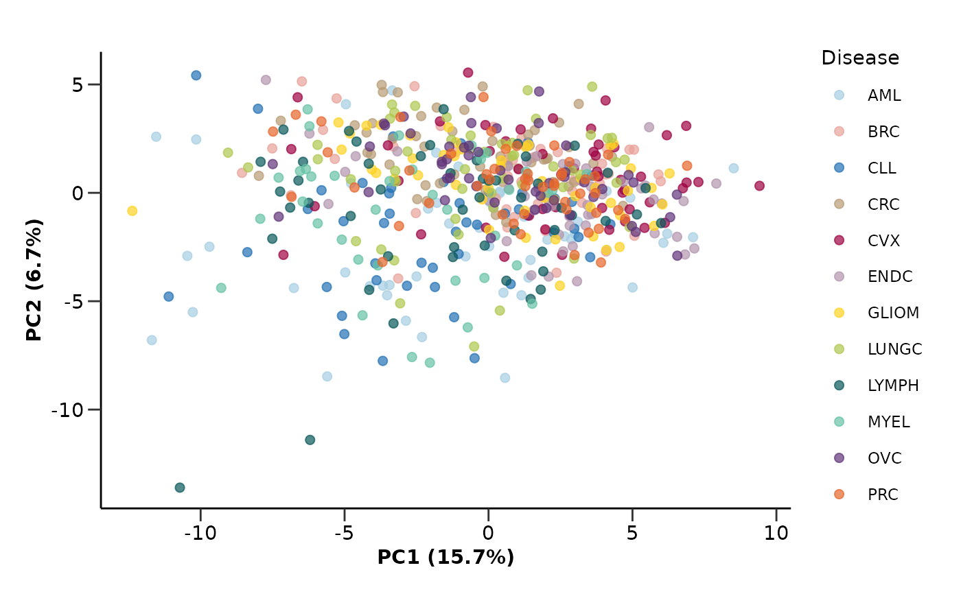
pca_plot: A ggplot object with the data points on the 1st and 2nd PCs plane.
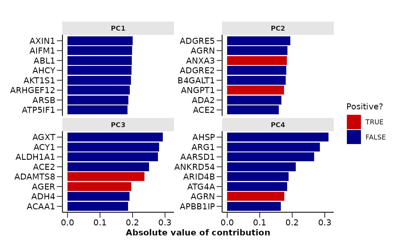
loadings_plot: A PCA loadings ggplot object.
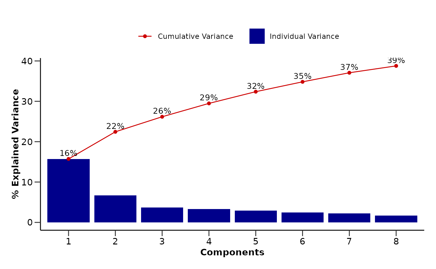
variance_plot: A ggplot object with the explained variance and cumulative explained variance.

Examples

do_pca(example_data,
       metadata = example_metadata,
       pcs = 8,
       wide = FALSE,
       color = "Disease",
       palette = "cancers12")
#> $pca_res
#> # A tibble: 586 × 9
#>    DAid        PC1     PC2      PC3    PC4    PC5     PC6     PC7    PC8
#>    <fct>     <dbl>   <dbl>    <dbl>  <dbl>  <dbl>   <dbl>   <dbl>  <dbl>
#>  1 DA00001  -3.67  -4.28   -2.34    -3.10  -2.65  -2.73   -2.78    0.433
#>  2 DA00002   4.11  -2.64    2.04    -0.441 -4.43  -1.91   -0.897   1.54 
#>  3 DA00003  -3.34   4.72    1.41     0.881 -0.561  0.308  -0.0612 -0.267
#>  4 DA00004  -4.78   0.443   1.41     0.107 -1.10  -0.262   0.350   3.33 
#>  5 DA00005  -4.98  -3.67    0.711   -5.70  -0.807 -3.77   -0.969   1.83 
#>  6 DA00006   0.395  0.0572 -1.90    -7.75   0.707 -2.70   -0.681   0.301
#>  7 DA00007 -10.5   -2.91   -0.382   -0.841 -1.61   1.96   -1.30    2.51 
#>  8 DA00008   2.64  -2.01    2.75    -0.128 -0.852  0.408  -1.70    0.595
#>  9 DA00009  -1.79  -0.461   2.79    -2.61  -2.71   0.0732 -3.08    1.75 
#> 10 DA00010   3.57   0.821  -0.00756  1.50  -2.66  -0.856   0.0190  1.17 
#> # ℹ 576 more rows
#> 
#> $loadings
#> # A tibble: 10,000 × 4
#>    Assay    Value PC    id       
#>    <chr>    <dbl> <chr> <chr>    
#>  1 AARSD1 -0.133  PC1   pca_EoYnc
#>  2 ABL1   -0.198  PC1   pca_EoYnc
#>  3 ACAA1  -0.163  PC1   pca_EoYnc
#>  4 ACAN    0.0123 PC1   pca_EoYnc
#>  5 ACE2   -0.0583 PC1   pca_EoYnc
#>  6 ACOX1  -0.135  PC1   pca_EoYnc
#>  7 ACP5   -0.0626 PC1   pca_EoYnc
#>  8 ACP6   -0.0933 PC1   pca_EoYnc
#>  9 ACTA2  -0.0751 PC1   pca_EoYnc
#> 10 ACTN4  -0.0424 PC1   pca_EoYnc
#> # ℹ 9,990 more rows
#> 
#> $pca_plot

#> 
#> $loadings_plot

#> 
#> $variance_plot

#>